Partial dependence

Partial dependence (PD) is the central interpretability tool for TSL. The key result is that for a separable model a 1D PD curve recovers the exact factor shape — not a contaminated main effect — so TSL's PD plots are model-native explanations rather than post-hoc approximations.

The problem with additive PD

The partial dependence of feature \(j\) is the marginal expectation

\[ \mathrm{PD}_j(x_j) \coloneqq \mathbb{E}_{X_{(-j)}}\bigl[m(x_j, X_{(-j)})\bigr]. \]

For an additive model with functional-ANOVA decomposition \(m(\mathbf{x}) = \sum_{S\subseteq[p]} m_S(\mathbf{x}_S)\) under the usual marginal identification constraint, the PD of \(x_1\) collapses to the intercept plus the main effect, \(\mathrm{PD}_1(x_1) = m_\emptyset + m_1(x_1)\), and therefore carries no information about any interaction term \(m_S\) with \(1\in S\) and \(|S|\ge2\). Strong interactions can leave no signature on the 1D PD at all (see the masked-interaction example).

Faithfulness for separable models

For a single separable product \(h(\mathbf{x}) = \prod_{j=1}^p h_j(x_j)\), marginalizing over the other coordinates leaves the factor shape intact up to a constant:

\[ \mathrm{PD}_j[h](x_j) = c_j\, h_j(x_j), \qquad c_j = \mathbb{E}\Bigl[\prod_{k\ne j} h_k(X_k)\Bigr]\ \text{constant in } x_j. \]

The interaction structure lives in the product form itself, so PD recovers \(h_j\) exactly rather than collapsing it to a main effect.

Proposition 1 — partial dependence decomposition

For a TSL estimator, fix a stage \(\ell\) and coordinate \(j\) and define

\[ c^{(\ell)}_{\pm,j} \coloneqq \mathbb{E}\Bigl[\prod_{k\ne j}\hat{m}_{\pm,k}^{(\ell)}(X_k)\Bigr], \qquad C^{(\ell)}_{\pm,j} \coloneqq c^{(\ell)}_{\pm,j}\,\lambda_{\pm}^{(\ell)}. \]

Then the 1D partial dependence of each signed branch factorizes into the factor shape times a constant:

\[ \mathrm{PD}_{\pm,j}^{(\ell)}(x_j) \coloneqq \mathbb{E}\bigl[\hat{m}_{\pm}^{(\ell)}(x_j, X_{(-j)})\bigr] = C^{(\ell)}_{\pm,j}\,\hat{m}_{\pm,j}^{(\ell)}(x_j). \]

Moreover, with \(\bar{m}_{\pm}^{(\ell)} \coloneqq \mathbb{E}[\hat{m}_{\pm}^{(\ell)}(X)]\) and \(Z_{\pm}^{(\ell)} \coloneqq \mathbb{E}\bigl[\prod_{j=1}^p \mathrm{PD}_{\pm,j}^{(\ell)}(X_j)\bigr]\), the stage admits an exact reconstruction from its 1D curves:

\[ \hat{m}_{\pm}^{(\ell)}(\mathbf{x}) = \frac{\bar{m}_{\pm}^{(\ell)}}{Z_{\pm}^{(\ell)}}\prod_{j=1}^p \mathrm{PD}_{\pm,j}^{(\ell)}(x_j). \]

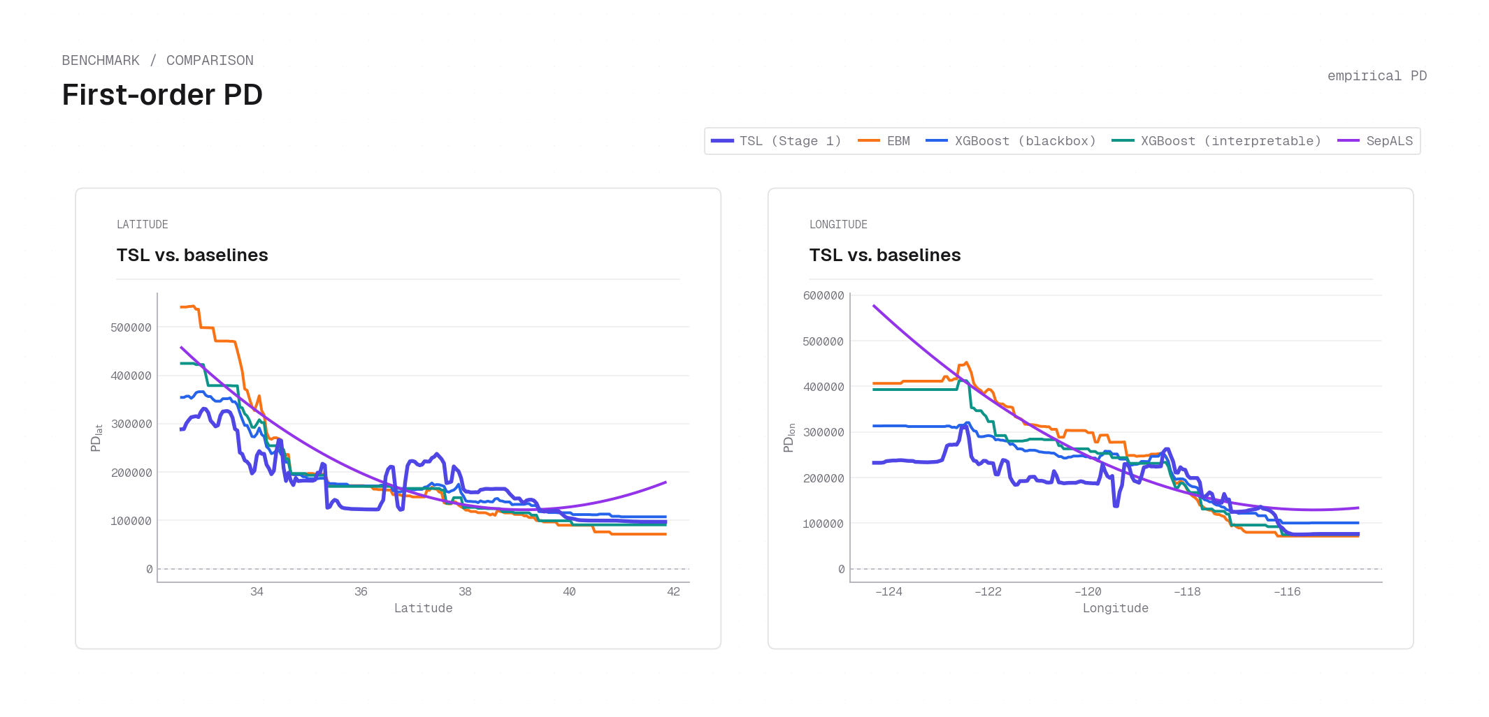
So each stage — and any explanation built from its factors — is recoverable from 1D PD summaries up to a single scalar normalizer per stage and sign branch. TSL's 1D PD plots therefore recover the fitted factor shapes (up to the constants \(C^{(\ell)}_{\pm,j}\)) without a surrogate.

California housing — TSL's summed \(\hat{m}_+\) branch PD for Latitude (left) and Longitude (right) compared with EBM, XGBoost (blackbox and interpretable), and SepALS. TSL (dark blue) preserves sharp localized peaks — a spike near lat 37–38 (Bay Area) and a concentrated coastal band near lon −122 — while the baselines smooth this into nearly monotone slopes. The faithfulness follows directly from Proposition 1: for a separable model, marginalizing over the other features leaves the factor shape \(\hat{m}_{\pm,j}(x_j)\) intact up to the constant \(C_{\pm,j}\), so the 1D PD curve is an exact scaled copy of the factor, not a contaminated main effect.

Implementation note — empirical marginalization

TSL.compute_partial_dependence_function (tsl-py/src/lib.rs) marginalizes over the empirical joint distribution of the other features, not a product-of-marginals reference, so the constants \(c^{(\ell)}_{\pm,j}\) are estimated correctly under feature correlation. The function returns, per stage, the \((C_+, C_-)\) constants and the curve values. The algebraic factorization holds for any reference distribution; only the statistical meaning of the average depends on that choice.

Backbone–tilt reconstruction from PD

The backbone and tilt can be read directly off the signed-branch PD curves (in the normalized gauge):

\[ b_j^{(\ell)}(x_j) = \bigl(C_{+,j}^{(\ell)} C_{-,j}^{(\ell)}\bigr)^{-1/2}\sqrt{\mathrm{PD}_{+,j}^{(\ell)}(x_j)\,\mathrm{PD}_{-,j}^{(\ell)}(x_j)}, \]

\[ d_j^{(\ell)}(x_j) = \tfrac12\log\!\frac{\mathrm{PD}_{+,j}^{(\ell)}(x_j)}{\mathrm{PD}_{-,j}^{(\ell)}(x_j)} + \gamma_j^{(\ell)}, \qquad \gamma_j^{(\ell)} = \tfrac12\log\!\frac{C_{-,j}^{(\ell)}}{C_{+,j}^{(\ell)}}. \]

The backbone is a magnitude summary that cannot cancel even when the signed stage PD \(\mathrm{PD}_j^{(\ell)} = \mathrm{PD}_{+,j}^{(\ell)} - \mathrm{PD}_{-,j}^{(\ell)}\) is near zero; the tilt captures the signed direction. Only the \((+)\) and \((-)\) PD curves per feature need be plotted to faithfully explain the model.

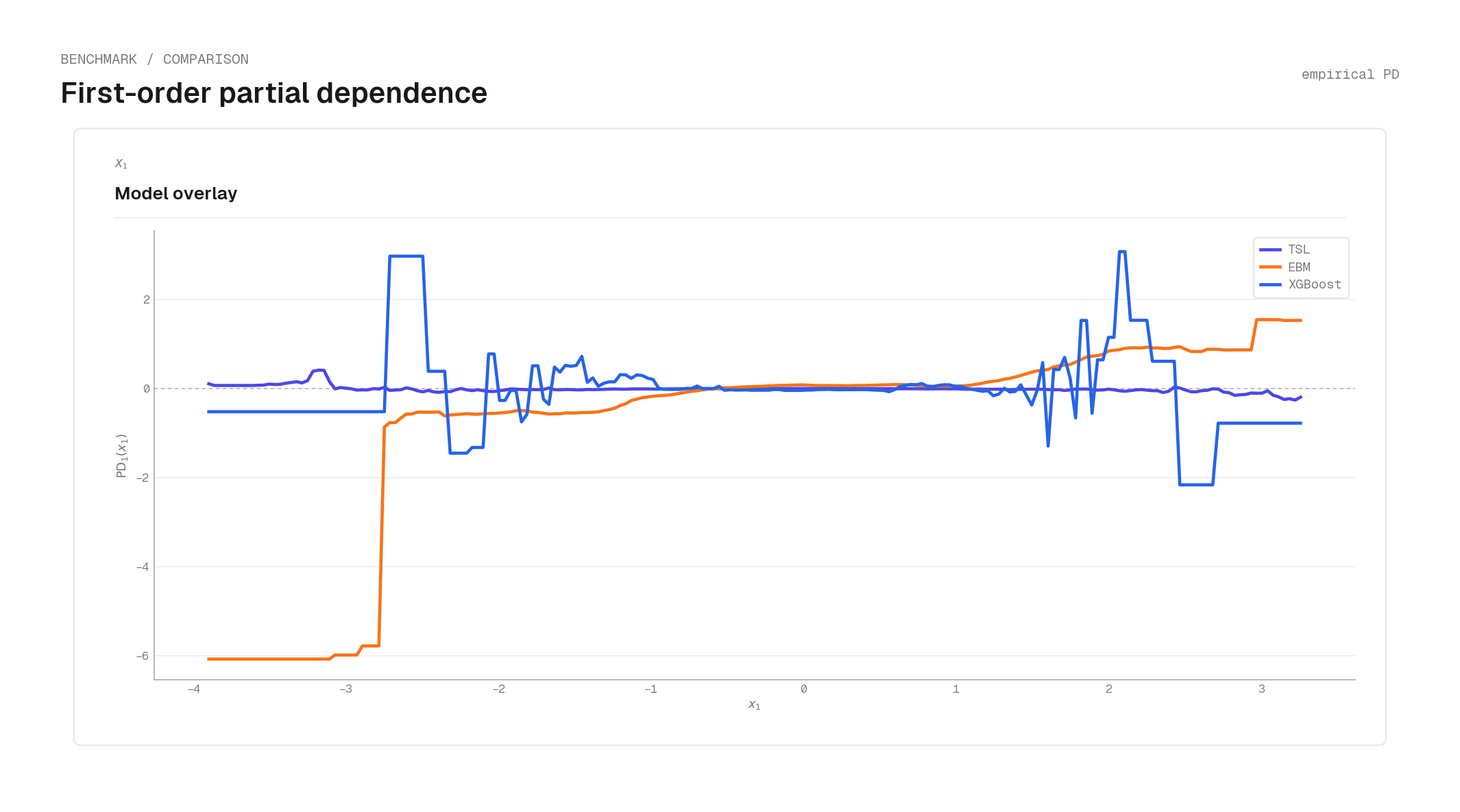
Signed-branch PD and the masked interaction

Consider independent features with \(Y = x_1^2\,x_2\,(1+x_3) + \varepsilon\) and \(\mathbb{E}[1+X_3]=0\). Then the population 1D PD of \(x_1\) is identically zero — \(\mathrm{PD}_1(x_1) = x_1^2\,\mathbb{E}[X_2]\,\mathbb{E}[1+X_3] = 0\) — even though \(x_1\) has a strong effect. Every model (TSL included) yields a near-zero 1D PD here, consistent with the population identity.

TSL's signed-branch PD escapes this trap: the backbone \(b_j^{(\ell)}(x_j)\) recovers the quadratic effect of \(x_1\) while the tilt stays small, so the magnitude is exposed even though the signed PD cancels. This is the practical payoff of the two-tensor form. The synthetic.py example reproduces the figure; see Examples.

Synthetic masked-interaction dataset (\(Y = x_1^2\,x_2\,(1+x_3)+\varepsilon\), \(\mathbb{E}[1+X_3]=0\)) — the signed 1D PD of \(x_1\) is near zero for every model (TSL, EBM, XGBoost), matching the population identity \(\mathrm{PD}_1(x_1)=0\). Yet the TSL-specific \(\hat{m}_+\) branch curve recovers the underlying quadratic shape of \(x_1\): the backbone \(b_j\) separates magnitude from sign, so the \(\hat{m}_+ \hat{m}_-\) product is large and quadratic even when the signed difference \(\hat{m}_+ - \hat{m}_-\) cancels. Reproduced by the synthetic.py example script.

Derived diagnostics

The Python layer builds several interpretation primitives on top of the PD math:

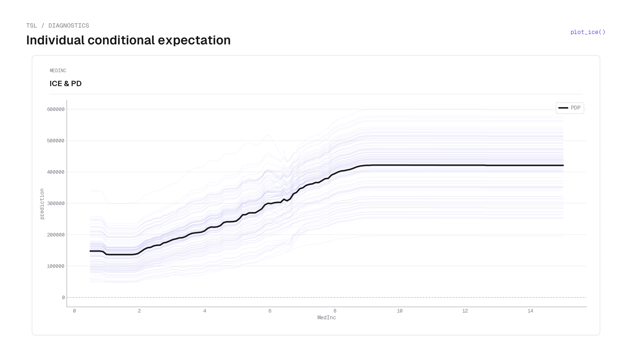
• ICE curves — compute_ice_curves traces individual conditional expectations (per-observation analogues of PD), scaled by scaling_plus/scaling_minus.
• First-order PD per feature — compute_first_order_partial_dependence_functions.
• Feature importance — variance-based backbone and tilt importance per stage, rolled up across stages by an energy weight into a combined score \(I_j\) (defined below).

Individual conditional expectation (ICE) curves on California housing for MedInc — each faint line traces one sampled observation's predicted price as MedInc varies while all other features are held fixed. The bold line is the average PD curve. The tight, upward-trending band shows that MedInc has a consistent positive direction across observations: every home benefits from higher income, but homes in high-value locations start from a higher baseline (vertical spread). ICE is the per-observation analogue of PD; see plot_ice for the API.

Feature importance

Feature importance reads off the backbone–tilt decomposition: a feature matters to a stage to the extent that its backbone (the magnitude gate) or its tilt (the signed direction) varies across the data. Evaluate the per-feature factors on the training sample \(\{x^{(i)}\}_{i=1}^n\) and take their empirical variances. For stage \(\ell\) and feature \(j\),

\[ I_j^{b,(\ell)} = \mathrm{Var}_n\!\bigl[\log b_j^{(\ell)}(X_j)\bigr], \qquad I_j^{d,(\ell)} = \mathrm{Var}_n\!\bigl[d_j^{(\ell)}(X_j)\bigr], \]

writing \(\mathrm{Var}_n[g] = \tfrac1n\sum_{i}\bigl(g(x_j^{(i)}) - \tfrac1n\sum_{i'} g(x_j^{(i')})\bigr)^2\) for the empirical variance over the sample. The backbone variance is taken on the log scale because the backbone enters the stage multiplicatively; under the normalization gauge \(\mathbb{E}[\log b_j^{(\ell)}] = \mathbb{E}[d_j^{(\ell)}] = 0\), so both are second moments about zero. A feature whose backbone and tilt are flat across the sample contributes nothing to that stage and scores zero.

Stages are then weighted by how much they actually move the prediction — their energy, the mean-squared stage contribution:

\[ \omega_\ell = \frac{E_\ell}{\sum_{k=1}^{R} E_k}, \qquad E_\ell = \bigl\lVert \hat{m}^{(\ell)} \bigr\rVert_n^2 = \frac1n\sum_{i=1}^n \hat{m}^{(\ell)}\!\bigl(x^{(i)}\bigr)^2, \]

where \(\hat{m}^{(\ell)} = \hat{m}_+^{(\ell)} - \hat{m}_-^{(\ell)}\) is the stage's signed contribution to \(\hat{m}\) (the per-stage OLS scalings scaling_plus/scaling_minus are folded in; see StagePredictor). The per-stage importances aggregate to global scores, and a single combined score folds the two channels together with a tilt weight \(\gamma \ge 0\) (default \(1\)):

\[ I_j^b = \sum_{\ell=1}^{R} \omega_\ell\, I_j^{b,(\ell)}, \qquad I_j^d = \sum_{\ell=1}^{R} \omega_\ell\, I_j^{d,(\ell)}, \qquad I_j = I_j^b + \gamma\, I_j^d. \]

compute_per_stage_feature_importance returns the per-stage grids \(I_j^{b,(\ell)}, I_j^{d,(\ell)}\), compute_aggregated_feature_importance returns the global \(I_j^b, I_j^d\) together with the weights \(\omega_\ell\), and compute_combined_feature_importance returns \(I_j\) — all rendered by plot_feature_importance.

All of these are plotted by the tensorsl.plot helpers — see the Plotting reference.