TSL — Tensor Separation Learning
TSL is a glass-box regression model: it fits accurately and lets you read its learned structure directly off one-dimensional plots — with no post-hoc surrogate. A fitted model is a small sum of stages, each a separable product of per-feature curves, so every feature's effect is recoverable exactly from a partial-dependence curve.
Everything below is produced by TSL itself (via the tensorsl.plot helpers) — these figures
are the model, not an approximation of it.
What TSL shows you
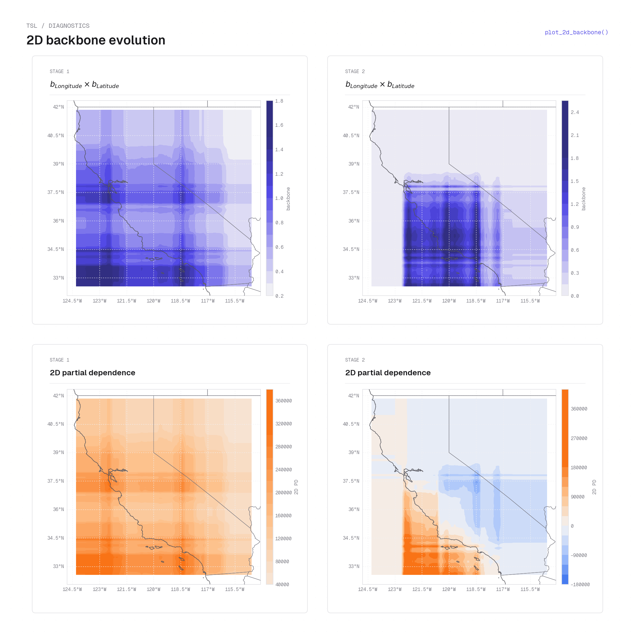
Where a stage is active — the spatial backbone
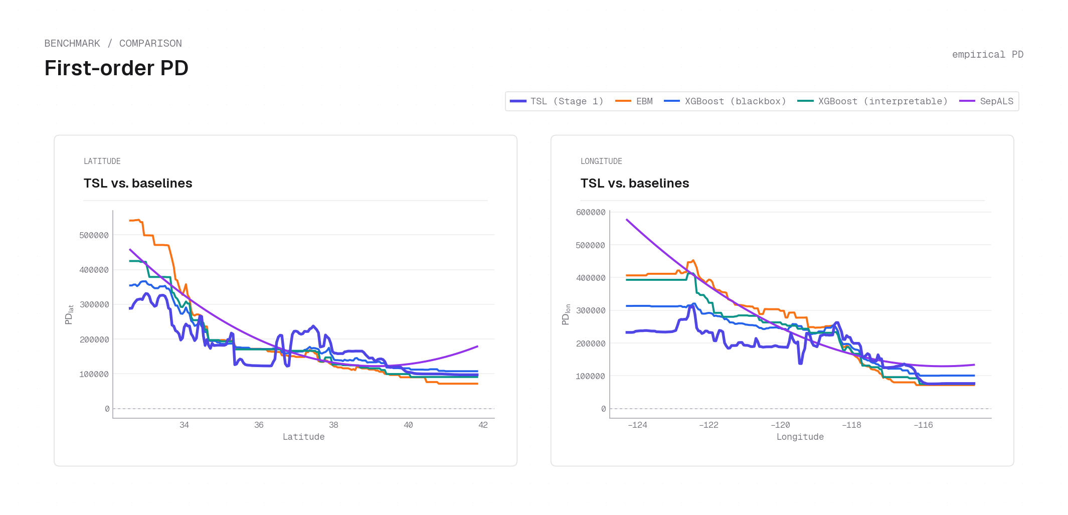
Faithful 1-D partial dependence
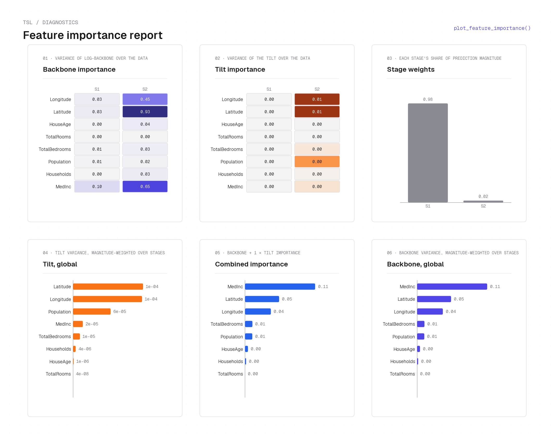
Feature importance — magnitude vs. direction
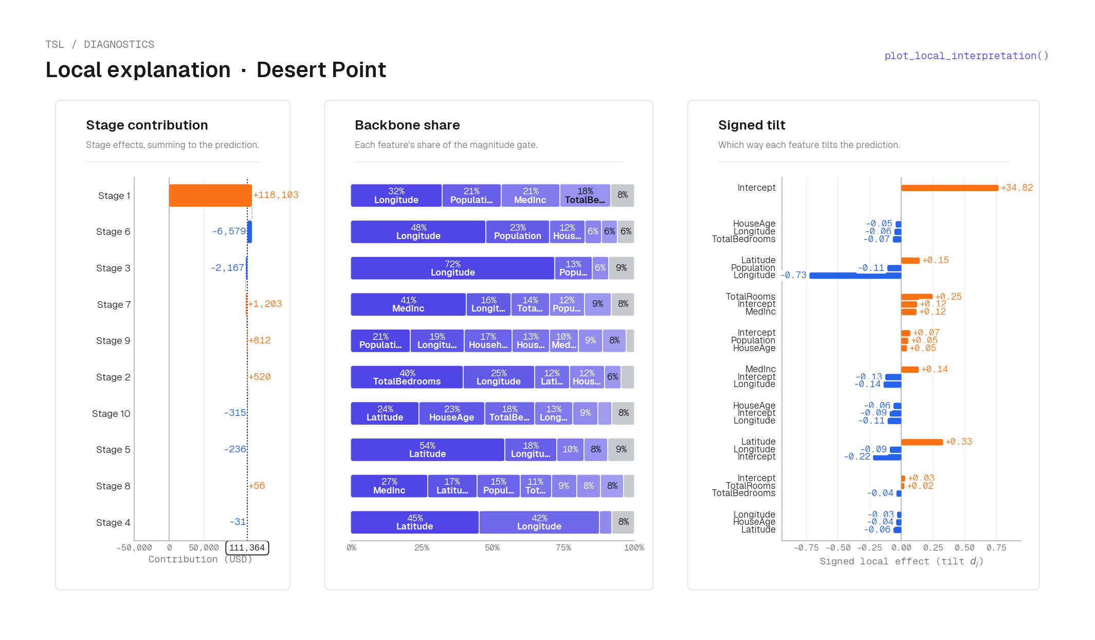
Local, per-observation explanations
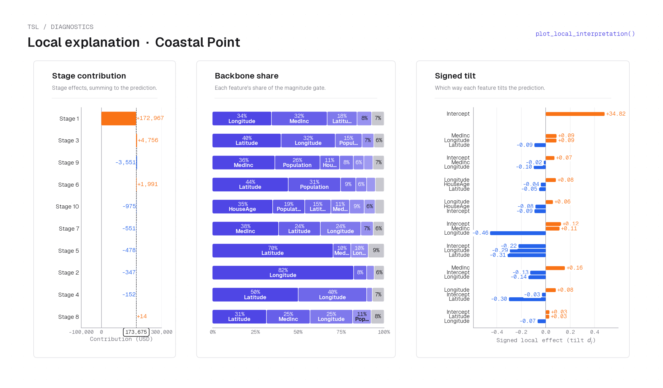
Read this first — it is short, and it is the point
These plots only mean something once you know what a backbone, a tilt, and a stage are. We strongly recommend reading the Under the hood section before relying on the figures: start with The model, then Partial dependence. It is what makes TSL interpretable rather than just another regressor.
Examples
The figures above come from runnable scripts in
tsl-py/examples/, which
reproduce the paper's plots via the tensorsl.plot helpers:
python tsl-py/examples/california.py
python tsl-py/examples/bike_sharing.py
python tsl-py/examples/synthetic.py
python tsl-py/examples/synthetic2.py
| Script | What it shows |
|---|---|
california.py |
spatial backbone, 1D PD faithfulness, feature importance, local explanations |
bike_sharing.py |
2D hour × workingday interaction PD |
synthetic.py |
the masked interaction — signed PD ≈ 0 for every model, yet the backbone recovers the effect |
synthetic2.py |
bagging diagnostics (backbone bimodality + similarity filtering) |
sepals_synthetic.py |
small synthetic factor-value / SepALS comparison |
Each script accepts --data-root, --out, --refit, and --variant; the pretrained
models in examples/models/ are used by default. See the
examples README for
the full per-script output list and flags.
How the codebase is organized
The model is a three-level hierarchy, and the src/ module tree mirrors it exactly:
| Level | Type | What it is | Docs |
|---|---|---|---|
| 1 | GridTensor |
one fitted separable component (backbone/tilt + \(\lambda_\pm\)) | GridTensor |
| 2 | StagePredictor |
one boosting stage: a bag of GridTensors + OLS scaling |
StagePredictor |
| 3 | TSL |
the boosted model: a Vec<StagePredictor> summed |
TSL |
The core is the Rust crate tsl_rust (library name tsl). tsl-py/ wraps it for Python
with a scikit-learn API (Python API), tsl-r/ (tensorsl) wraps it for R
with an S3 fit/predict interface and a ggplot2 interpretability layer
(R API), and tsl-split-evolution-dashboard/ (tslviz) visualizes how a
fit was built (Visualization dashboard).
Where to start
Before anything else, read the Under the hood material — start with Notation and The model to understand what a backbone, a tilt, and a stage are. That understanding is what makes TSL interpretable rather than just another regressor, and it is worth five minutes before you fit your first model. From there: Fitting and Partial dependence round out the theory.
- New to TSL? Getting started — install, fit, predict.
- Using the model? The Python API or R API, the Hyperparameters reference, then Examples.
- Working on the code? Start with Architecture and its two critical invariants, then the per-module pages.